Mass or Weight?

Hello again!

I know my blog is called Algebra Demystified, but today, I’d like to talk about a physics concept – the difference between mass and weight.

First, let me note that the strict definition of the terms mass and weight is rather rigorous, not to mention the fact that there are several types of masses and weights. Since this blog is meant to be engaging and simple, I’ll instead give you the most important facts.

Mass and Weight are Not The Same!

One of the most common (if not the most common) mistakes people make is substituting mass for weight, and vice versa. This is perfectly O.K. in a casual setting, but the exact sciences require exact definitions.

For starters, mass is a physical property of the object. By physical I mean that an object’s mass depends on the object itself, not on the environment in which it is located. So, for example, my mass (yes, mass, not weight) is 50 kg. If I go to the moon, my mass will still be 50 kg. Same thing if I go scuba diving. The external conditions that an object is subjected to don’t affect its mass in the slightest.

Weight, on the other hand, is a force. Think of a force as something “pushing” or “pulling” on an object. So, just from this informal definition, it’s obvious that you can change a force. And yes, an object’s weight does change, depending on the environment.

What is Mass?

Put simply, mass measures the amount of material in an object. So, for example, a basketball has more material in it than a golf ball, and so has greater mass. As I said above, you cannot change the mass of an object by changing the forces exerted on it. That’s because an object is composed of the same material (i.e. atoms and molecules), whether it’s located on Earth or somewhere in an alien galaxy during a zombie apocalypse.

More formally, mass represents an object’s resistance to acceleration when a force is applied.

Sounds complicated? Let me illustrate.

Let’s put a golf ball on an ice ramp. Now let’s push the ball. Even though the force you apply is small, the ball rolls freely. Its resistance to acceleration (or inertia) is small. A small push gets the ball rolling – literally.

Now let’s do the same experiment with a car. Maybe some of you will manage to perform the feat, but when I push on a car, it doesn’t move. No matter how hard I push, the car remains still and doesn’t move an inch. It “resists” your push, and very much at that.

Why could I push the golf ball freely, and the car not at all?

Because the golf ball resisted the force I applied only slightly. The car, on the other hand, resisted way stronger. So, the car has greater mass than the golf ball.

What is Weight?

As I mentioned earlier, weight is just a force. More specifically, it is the force exerted on an object by gravity. That’s as simple as it can get. There are other definitions, as well, but they are more specific. Almost always, when you come across “weight” in physics, it will mean the force on an object due to gravity.

Remember I said that weight and mass are not alike? Well, there is a formula that relates them:

W = mg

You may have noticed it is a slight variation of Newton’s second law,

F = ma

However, the first formula is just a specific example of Newton’s second law, where the acceleration in question (the a in the second equation) is the force of gravity.

And… The Units, Please?

When speaking about physical concepts, one of the biggest questions is what units do we use. For example, when we speak about time, we don’t say:

It took me 23 reading this book.

We say instead:

It took me 23 hours reading this book.

Same with mass and weight.

The unit of mass is the kilogram (kg.) You’re probably familiar with this unit already, since it’s used in everyday life.

And the unit of weight is the newton (N) Just in case you don’t know, a newton is defined as the force needed to accelerate 1 kg. of mass at the rate of 1 m/s2 in the direction of the applied force.

And that’s all there is to it! Until next time!
Degrees of Smoothness

All images in this blog post taken from Google.


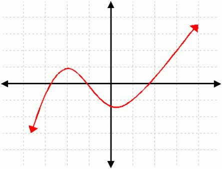
In my previous blog post, I brought up the topic of smoothness. We saw that a function is not smooth if its derivative cannot be expressed by another continuous function. For example, the derivative of the absolute value function, |x|, we discussed in the last post was not continuous; and therefore, |x| isn’t smooth.

What if we can express the derivative of a function as a continuous function? Does this make the function smooth? To answer this question, let’s examine the function y = x|x|.

The derivative of this function can be expressed as a continuous function. In fact, it’s the absolute value function, 2|x|, which is continuous. However, when we try to find the second derivative (derivative of the derivative) of the function, we fail to derive a continuous function. (In fact, we’ve shown this result in the last blog post).

So, we’ve only found the first derivative. That means that our function, x|x|, has a smoothness of order 1. Mathematically, we say that it’s a class C1 function.

Let’s examine a similar function, x2. Let’s try to calculate its derivatives:

  1. f'(x) = 2x
  2. f”(x) = 2
  3. f”'(x) = 0
  4. f””(x) = 0

We can differentiate this function indefinitely. Therefore, we say that the function belongs to the class C.

Now, here’s the question. Which of the functions we examined are smooth?

Well, the term “smooth” doesn’t have a rigorous definition. People use it in two ways:

  1. Meaning that the function is smooth enough for what they need to do with it,
  2. Meaning that the function is indefinitely smooth, belonging to the class C.

Therefore, it’s more correct to specify the degree of smoothness of a function, rather than simply saying that the function is smooth or not.

I hope that this post was informative as well as engaging. As always, if you have any ideas about future posts, or just to express your ideas or doubts, feel free to comment.

Till then!

Exploring Smoothness and Continuity

All images in this blog post taken from Google.


No doubt you have heard of the terms smooth and continuous when referring to functions. In this blog post, I’ll try to explain what these terms really mean; as usual, in the most informal language possible.

continuous function is a function that you can trace with a pencil without lifting it off the paper. This is a continuous function:

alg2_vertlinetest

Now, if at least one of the following are true, the function is not continuous:

  1. At some point, you have to lift your pencil and move it to some other spot on the function to continue the movement,
  2. At some point on the graph, the function is not defined (it has a hole).

Smoothness is a similar, but not identical, concept. It is closely related to the concept of derivatives that I mentioned in my post Derivatives Demystified, so I’ll be leveraging that post to help us understand smoothness.

Basically, for a function to classify as smooth, it should have a derivative at all points of the graph. I won’t go into the calculus definition (I might scare you out of calculus altogether); I’ll instead use the analogy I gave you in the post above.

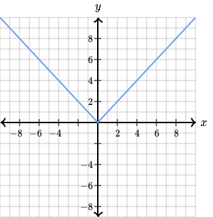
Here’s an example of a function that is not smooth:

3b9b8f4b4dac19e1197e9dd94553d0822f9fe69a

That’s the familiar absolute value function:

y = |x|

Why is this function not smooth? Well, let’s consider the point x = 0.

Graphically, this function has a steep turn at this point.

Analytically, this means that the function has no derivative at this point and, consequently, is not smooth.

Why is that?

Let’s say that we’re moving from the far left of the function to the far right and examine the derivative of the function at each point as we pass through it. I hope that by now, you remember that the derivative is just the slope of the function at the point of interest. Nothing advanced. Just easy high school algebra.

We find that for negative values of x, the derivative of the function is -1.

However, for positive values of x, the derivative is +1.

We cannot derive a formula that can calculate the derivative at any point. If we use -1 as the formula, we will get the wrong answer for all positive values of x. If we use +1 as the formula, we will be mistaken on all negative values. Any attempts to find any relationships between y and x don’t work, either.

So, the function isn’t smooth.

Now that we can recognize a function that is not smooth, can we just call it a day and say that all other functions are smooth?

Well, not really…

You see, smoothness is not a black-and-white concept. You cannot say that a function is either smooth or not. Mathematicians refer to so-called degrees of smoothness. That will be the topic of our next blog post.

Until then!

Derivatives Demystified

Welcome back! Today I’m returning with a new post on calculus, this time concerning derivatives. If you’ve read my series on limits, I hope you realized that calculus isn’t that scary, after all; in fact, it’s fun and exciting!

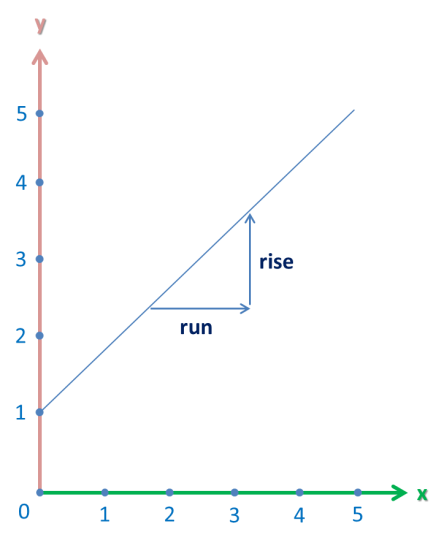
Let’s start with a quick talk on slopes of linear equations. You probably know from algebra that the process of determining the slope of a line is very easy. You simply select any interval and divide the vertical change (a.k.a rise) by the horizontal change (a.k.a. run). I illustrated this below:

deriv-1

One crucial detail is that the choice of the interval doesn’t matter. The slope of a line will remain the same whether you choose the whole range (e.g. from -∞ to ∞) or a small interval (e.g. from -1 to 2).

How about if we shift this definition of a slope to other graphs. Let’s take parabolas, for example. We can take an interval on this parabola and use the formula above. So, apparently it’s easy and it works!

Or does it?

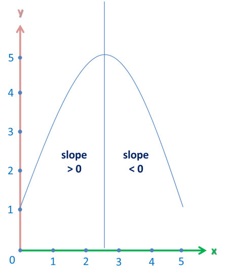
Unlike linear equations, the slope of parabolas constantly changes. I illustrated one example below:

deriv-3

If you take an interval from the left half, the slope will be positive. However, intervals from the right have will have a negative slope.

So, that means that slopes of non-linear equations make no sense?

Well, let’s loosen the definition a bit.

Let’s represent the slope not by a number, but by a function. This function will tell us the slope of a graph at a particular point. Thus, even though all points on the graph will have different slopes, the slope operation suddenly makes sense.

And this function is called the derivative and is denoted f'(x), read “f prime of x”.

I’ll examine methods of calculating the derivative of functions in subsequent posts, but now I’ll give you a quick example.

The derivative of the quadratic function x2 is 2x. What does that mean?

Well, that means we can calculate the slope of x2 at any point just by plugging in the x-coordinate into 2x, the derivative.

For example, the slope of x2 at x = 3 is:

f'(3) = 2 * 3 = 6

and the slope at x = -5 is:

f'(-5) = 2 * -5 = -10

It’s really that easy!

Now, you might wonder, do linear functions have derivatives? Well, turns out they do! The derivative of linear functions is just a constant and is equal to the slope of the line.

So, the slope of the linear function 5x at the point x = 7 is:

f'(7) = 5

So, the derivative (a.k.a. slope) of a line doesn’t depend on the point, which rephrases what I said earlier in the post.

I hope you found this post informative and fun to read. If you have any questions or suggestions, feel free to comment.

Next time I’ll probably return with another calculus post. You may think that the easy-going nature of my posts is due to the fact that limits and derivatives are introductory material, but if you have the attitude, you’ll breeze through all of calculus easily 🙂

Until then,
Vladimirr Petrunko

Limits Demystified (Part 2)

Welcome back! If you’ve read my last post Limits Demystified (Part 1) I hope you realized that calculus isn’t that scary. In fact, according to my personal experience, limits are in fact easier to comprehend than many Algebra 1 topics. Absurd but realistic.

Limits Tending to Infinity

Okay, maybe the mere word infinity turns you off. Well, think of it this way. When you move along the real number line starting from the origin and go right, you pass the numbers 1, 2, 3, 4… If you pass further, you will encounter bigger numbers: a thousand, a million, a billion… Well, what if you went all the way forever? That’s infinity.

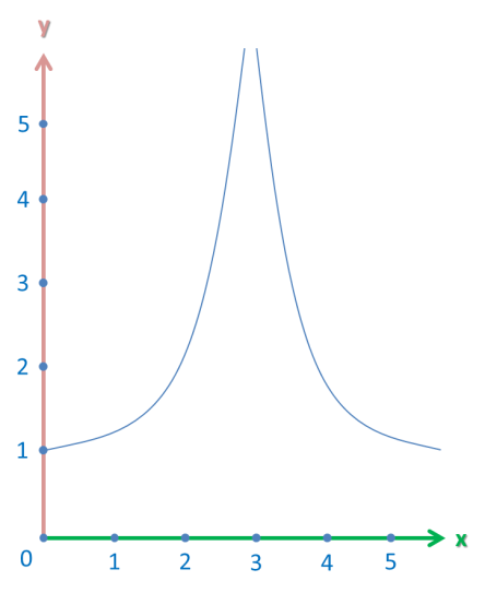
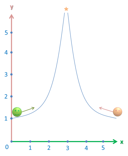
So, let’s take a look at the following graph:

graph-8

We want to find the limit of this graph as x approaches 3 from both sides.

Now, you probably remember what we do when we encounter limits – we imagine two people and a roller coaster ride:

graph-7

However, this graph has a vertical asymptote at the point x = 3. This is just a fancy line for a vertical line that the graph approaches, but never actually reaches.

That means that both people will never reach the meeting point, since I just said that the graph never actually reaches it. So, what is the limit at that point?

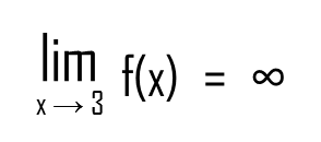
Let’s imagine that the meeting point is a point – infinity. So both people are heading toward that point, albeit forever. That means that the graph tends to infinity at that point, or:

lim-9

However, this is only one school of thought. Other mathematicians have decided that since infinity is not a defined point, the graph doesn’t even have a limit there. It’s up to you to decide, but now you know that the above situation is rather equivocal. However, both representations are correct – the limit-to-infinity representation and the limit-is-undefined one.

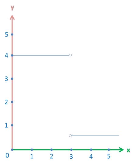
And, to close off the discussion on limits, one final graph:

graph-1

This graph isn’t defined at the point x = 3. What is the limit of the function as it approaches 3 from the left; from the right; from both sides?

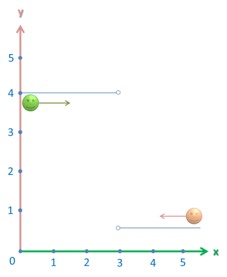
Now this question is a bit more complicated than our previous graph. However, our faithful friends come to our assitance:

graph-2

When the person in green (on the left) reaches the meeting point, he says that it’s located at the y-coordinate of 4.

However, the person on the right reaches the meeting point and disagrees. “It’s located at y-coordinate of 1″, he says.

Who’s right? Well, both of them. The limit from the left and the right are different, however, they are limits. (Again, it doesn’t matter if the function is defined there or not. It’s just how the function looks).

Let’s write it in mathematical language:

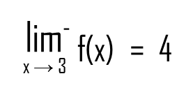
lim-5

The minus sign on top of the lim simply means that x is approaching 3 from the left.

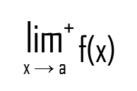
And from the right:

lim-3

I guess you got the meaning of the plus sign. Here, x approaches 3 from the right.

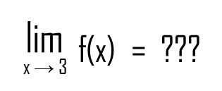
However, the two limits are different. Which do we choose for the from-both-sides limit?

lim-8

Well, it’s simple. No calculations, no advanced techniques. If the two limits aren’t equal, the function doesn’t have a from-both-sides limit. It’s undefined.

lim-7

So, we’ve analyzed our fourth function and with this, I conclude this chapter on limits.

Any questions / tips / suggestions are welcome in the comments, as usual.

Until then,
Vladimirr Petrunko

Limits Demystified (Part 1)

Welcome back! It’s been a long while since I last wrote a post here… Today I’ll delve into the realm of calculus! One of the reasons for this decision is the “calculus-o-phobia” that surrounds modern students. I’d like to examine the basic tenets of calculus step by step and show that it’s really that easy!

As always, I won’t use textbook definitions or complicated formulas, just layman’s terms. However, this blog post is a bit lengthy so, if you like, you might want to tackle it in several sittings. So, are you ready?

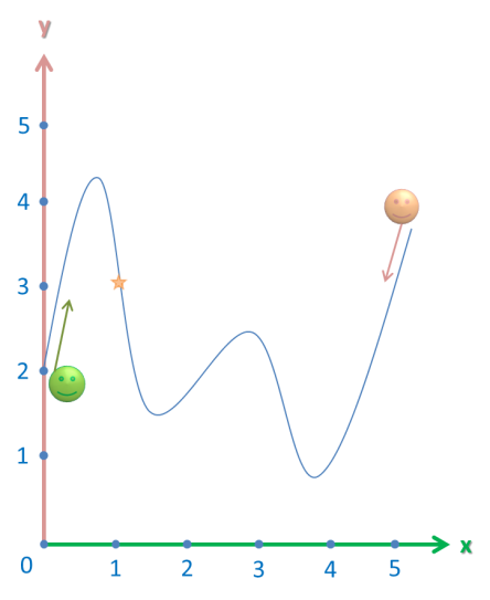
Let’s start with a function:graph-1

Let’s find the limit of this function as the variable x approaches 1.

To do this, let’s imagine two people approaching the x-value of 1 (the “meeting point”) from opposite ends of the graph along the function like on a roller coaster ride. The following illustration shows what I mean:

graph-2

Those two people just go with the flow. They don’t know how the function was defined – whether it’s a quadratic, cubic equation or a piecewise graph. They simply slide along the waves of the graph, ignorant of the mathematics behind this.

When the person on the left (in green) reaches the meeting point, he tells the y-coordinate of the point (in this case 3). To rephrase this in mathematical terms,

The limit of our function,
as x approaches 1 from the left,
is 3.

Note the key words – from the left. For now, we don’t care about the part of the graph to the right of the meeting point. We’re only interested in the left part.

The person on the right (in orange) does the same. Since the graph is continuous, he also finds that the y-coordinate is 3. Or,

The limit of our function,
as x approaches 1 from the right,
is 3.

Now, if the limit from the left and right at a given point are equal, then we say that the function has a limit at the point. So, according to this definition,

The limit of our function,
as x approaches 1,
is 3.

Which basically means: the y-coordinate of the meeting point (located at = 1) of two people, arriving from opposite ends of the function, travelling along its graph, is 3.

You may have noticed that the value of the function at our meeting point is also 3. That’s not surprising, since our function is continuous and it doesn’t really matter whether we take the y-coordinate of the meeting point directly or arrive at the point from opposite ends of the graph.

Or does it?

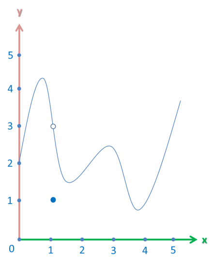
Let’s take this function:

graph-3.png

It’s almost the same as the previous function. However, unlike in the previous example, our smooth graph has a discontinuity at our meeting point. The function is defined there, though, but is equal to 1 instead of 3.

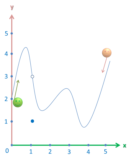
However, when we ask our two faithful friends to come together from opposite ends of the graph, we notice that they both say that the x-coordinate of their meeting place is 3. Just as before, they take a roller coaster ride:

graph-4

They have absolutely no way of knowing that someone “removed” the point (1, 3) from the list (xy) coordinates of the graph. Again, they don’t know how the function is defined. They simple ride the graph like a roller coaster.

But when they come to the meeting point, they notice something weird… The function isn’t defined at 3, it’s defined at 1. However, the function still has a limit there, and – more importantly – the limit is still equal to 3.

Just a bit of Mathematical notation…

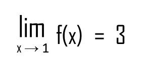
I haven’t used a single formula yet in my blog post (and that’s good, in fact). I guess, just for the sake of mathematics, I need to show you how to write a limit formally. You won’t be rambling about people and roller coasters in Calculus class. I mean, you might do that, but it’s only for your own understanding. Here’s how you would write it on paper:

lim-4

Which just means, as x approaches 1 from both sides, the y-coordinate approaches 3.

In the next blog post I’ll take a look at several other kinds of limits – limits that tend to infinity and limits that do not exist.

Until then,

Vladimirr


Moving to a Different Format

Hello, guys! Sorry I’ve not posted a while. Y’know, I’ve decided to take a big step in the growth of my blog, and from now on the vast majority of my blog posts will be in a video format. I have a playlist on my YouTube channel dedicated to mathematics, I’ll be uploading my math videos there.

I haven’t forgotten about matrices, I plan to make several videos about that soon. I believe that complicated topics like matrices merit their own videos, because it’s kinda difficult to explain the intricacies of advanced math in text.

Here’s my first video, where I explain a very simple way to help you remember the values of sine and cosine of 30, 45 and 60 degrees – the main angles you’ll find in geometry and trigonometry: https://www.youtube.com/watch?v=7qxfxUkpmcc Hope you like it!

See you soon!

Matrices: More Powerful Than You Think!

Hello again! Today, and for several blog posts at least, I’ll discuss a whole new topic: matrices. They may look like simple structures on first glance, but in reality, they are very intricate, and also very powerful and find their use in many areas of modern mathematics.

Simply put, a matrix is just a table of numbers, organized into (horizontal) rows and (vertical) columns. Here is a simple matrix, that contains 3 rows and 3 columns:

1 2 3
4 5 6
7 8 9

(We usually indicate matrices by a letter, such as A, in this case).

We indicate a particular element of a matrix by two subscripts, one representing the row number, and the other – the column number. So, in the matrix above, the element 6 lies in the position A2,1. What this means is that 6 is located in row 2, column 1.

Let me examine some basic matrix operations first:

Addition (subtraction)

First, let me note that subtraction is the inverse of addition, so, for any two matrices,

A – B = A + (-B).

To switch the sign of a matrix, you simply switch the sign of each of its elements.

You can only add matrices that have the same number of rows and columns. Otherwise the whole operation is illegal.

Let’s say that A and are two such matrices and let C be their sum.

For every pair of indices i,j:

Ci,j = Ai,j + Bi,j

In other words, we simply add the elements of both the matrices at a given position.

Multiplication

Before we go on any further, let me point out one important thing – the multiplicative inverse of a given matrix is not trivial to calculate, unlike the additive inverse. In other words, we won’t be considering division in this post, because calculating the inverse is a whole new topic, which I won’t have sufficient time to explain in this post.

First, let’s examine how we would multiply two matrices, where one of the dimensions is 1, together. I like to call them thin matrices, since they consist of only one row (or column). Here’s the method:

{A, B, C} * {D, E, F} = AD + BE + CF

We multiply the first element of A by the first element of B, the second element of A by the second element of B, and so on. All of those products get added up in the end.

So, when we multiply a row and a column, the result is a single number (called the dot product), not a resultant matrix. Let’s take an example:

{2, 8} * {-1, 6} = 2(-1) + 8(6) = -2 + 48 = 46

Let me note that the two matrices should have the exact same number of elements in its single row. Only then is the multiplication legal.

Now let me show you how we would multiply matrices of any dimension.

Let A be a a * b matrix, and let B be a c * d matrix. The multiplication is legal if and only if  b = c , in other words, if A has as many columns as B has rows.

The rest is relatively simple. Let C be the resultant matrix; it has dimensions a * d . For every pair of indices i,j:

Ci,j = Ai * Bj

From the matrix A we take the row with index i, from the matrix B – the column with index j. We then get their dot product and place it in the new matrix in the position i,j.

One curious aspect of multiplication is that the commutative property is not always fulfilled. That means that AB does not always equal BA. Sometimes one of them may not even be defined (i.e. legal), or, even if it is defined, their values might not be equal.

The Identity Matrix

There’s a special kind of matrix – the identity matrix, in which all the elements are 0, except for the ones where the row number equals the column number. Here’s an example of an identity matrix:

1 0 0
0 1 0
0 0 1

These are the matrix fundamentals, which we’ll be using in the next blog post, where I’ll talk about how to apply matrix addition and multiplication to solve linear systems of equations!

Feel free to post any questions related to the topic in the comments! Until then! 🙂